Things about Vlookup In Excel
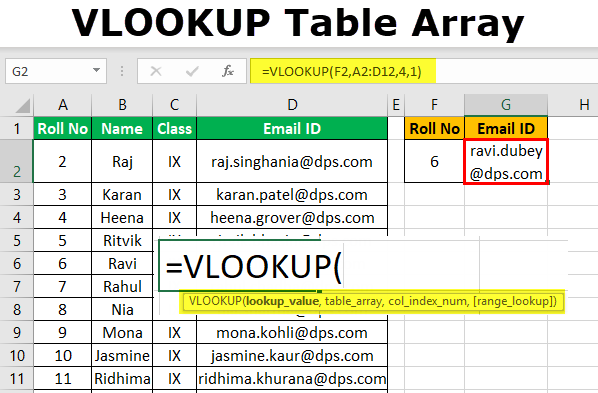
What does it do? Look for a value in the very first column of a table variety and returns a value in the exact same row from one more column (to the right) in the table range. Formula failure: =VLOOKUP(lookup_value, table_array, col_index_num, [range_lookup] What it suggests: =VLOOKUP(this value, in this listing, as well as obtain me value in this column, Exact Match/FALSE/0] Excel's VLOOKUP feature is probably the most pre-owned feature in Excel yet can likewise be the most challenging one to understand.
You will certainly be making use of VLOOKUP with self-confidence hereafter tutorial! ACTION 1: We need to go into the VLOOKUP feature in a blank cell: ACTION 2: The VLOOKUP arguments: What is the value that you intend to try to find? In our initial example, it will be Laptop computer, so pick the Product name What is the table or range which contains your data? See to it to select the stock listing table to ensure that our VLOOKUP formula will certainly browse right here Guarantee that you push F 4 to make sure that you can lock the table array.
Apply the very same formula to the remainder of the cells by dragging the reduced appropriate corner downwards. You currently have every one of the outcomes! Exactly how to Use the VLOOKUP Solution in Excel HELPFUL SOURCE: .
Updated: 11/16/2019 by Computer Hope HLOOKUP and also VLOOKUP are functions in lookup table. When the VLOOKUP feature is called, Excel look for a lookup value in the leftmost column of an area of your spreadsheet called the table range. The feature returns an additional worth in the same row, defined by the column index number.
Our Vlookup In Excel Diaries
The V in VLOOKUP means row). Allow's use the workbook listed below as an example which has two sheets. The first is called "Information Sheet." On this sheet, each row has details about a stock item. The initial column belongs number, and the third column is a cost in bucks.
In the screenshot below, cell B 2 is chosen, as well as its formula is provided in the formula bar on top of the sheet. The worth of cell B 2 is the formula =VLOOKUP(A 2,'Data Sheet'!$A$ 2:$C$ 4,3, FALSE). The above formula will certainly populate the B 2 cell with the rate of the component identified in cell A 2.
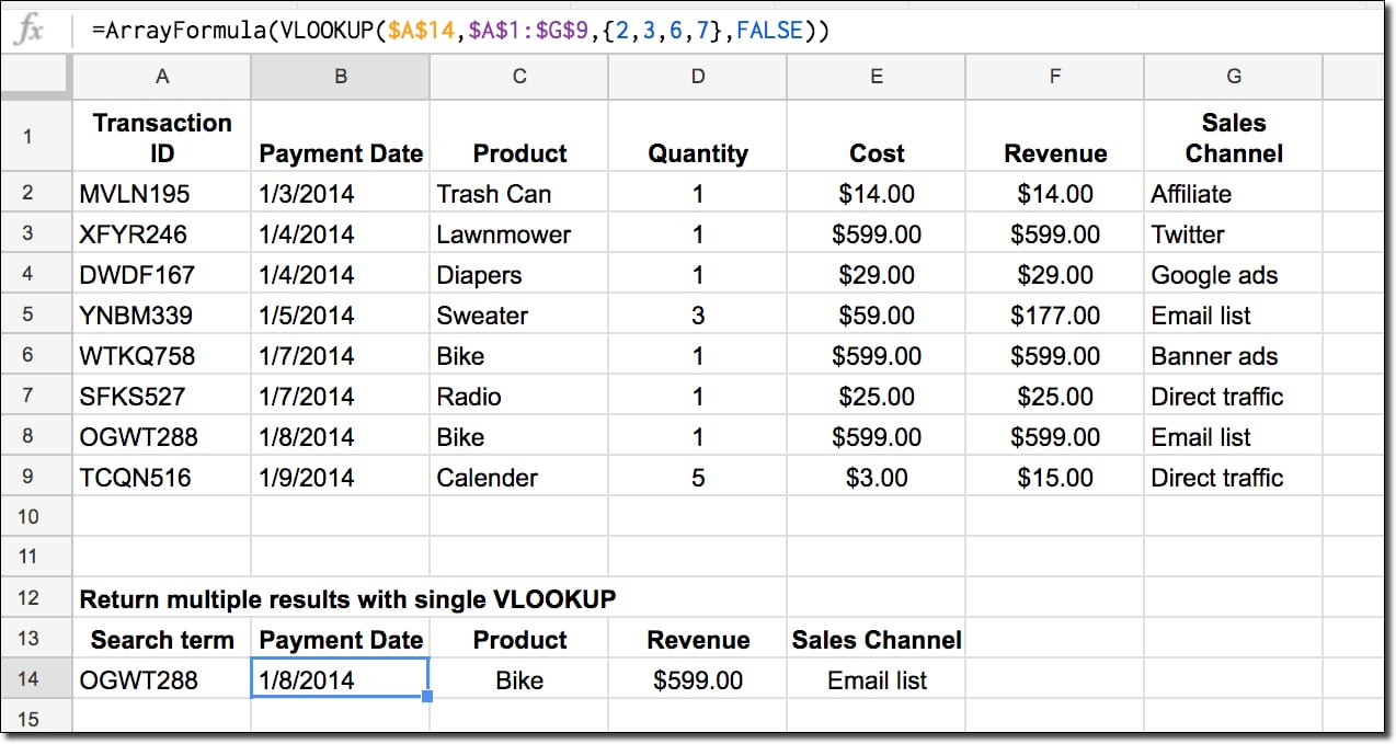

In a similar way, if the part number in cell A 2 on the Lookup Sheet adjustments, cell B 2 will automatically upgrade with the price of that part. Allow's take a look at each aspect of the example formula in much more information. Formula Aspect Meaning = The amounts to indication (=-RRB- shows that this cell includes a formula, and also the result must become the worth of the cell.
( An opening debates to the function. A 2 A 2 is the cell having the value to seek out. 'Information Sheet'!$A$ 2:$C$ 4 The second argument, the table selection. It defines a location on a sheet to be made use of as the lookup table. The leftmost column of this area is the column which contains the Lookup Worth.
Rumored Buzz on How To Vlookup
Specifically: Sheet Call is the name of the sheet where the table range (search location) lies. It must be confined in solitary quotes (' ') and complied with by an exclamation mark (!). A sheet identifier is required only if you're searching for information on one more sheet. If you omit the sheet identifier, VLOOKUP will certainly attempt to carry out the lookup on the same sheet as the function itself.
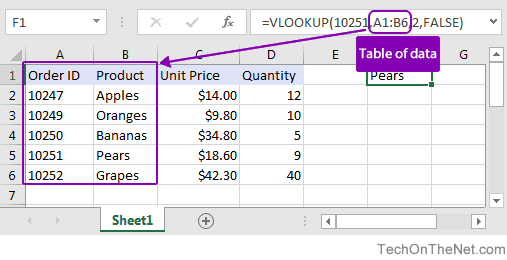
Each worth is come before by a buck sign ($), and also a colon (:-RRB- is used to separate the upper-left and lower-right collections of values. The leftmost column of the table array must include your lookup value. Always specify your table selection so that the leftmost column includes the value you're looking up.
3 The third VLOOKUP debate, the Column Index Number. It represents the variety of columns, offset from the leftmost column of the table variety, where the result of the lookup will be found. For instance, if the leftmost column of the lookup range is C, a Column Index Variety Of 4 would certainly show that the result needs to come from the E column.
A is the very first column, B is the second column, and C is the 3rd column, so our column index number is 3. This debate is needed. FALSE The fourth debate is the Array Lookup worth. It can be either REAL or FALSE, and also it defines whether Excel must do the lookup making use of "precise lookup" or "variety lookup".
The Basic Principles Of Vlookup Function
A fuzzy mage suggests that the beginnings at the leading row of the table array, browsing down, one row at a time. If the worth because row is less than the lookup worth (numerically or alphabetically), it continues to the following row and also attempts once again. When it locates a value higher than the lookup worth, it quits browsing as well as takes its result from the previous row.
A precise suit is called for. If you're not exactly sure which kind of suit to make use of, pick FALSE for an exact suit. If you choose TRUE for a range lookup, see to it the information in the leftmost column of your table array is arranged in rising order (least-to-greatest). Otherwise, the outcomes are inaccurate.
If you omit this argument, a precise lookup will certainly be executed.) A closing parenthesis, which suggests completion of the disagreement list and completion of the function. The lookup worth have to be in the leftmost column of the table variety. Otherwise, the lookup feature will certainly fail. Ensure that every worth in the leftmost column of the table selection is distinct.
Excel IFERROR with VLOOKUP (Tabulation) IFERROR with VLOOKUP in Excel Exactly How to Make Use Of IFERROR with VLOOKUP in Excel? Pros & Cons of IFERROR with VLOOKUP in Excel To learn about the IFERROR with VLOOKUP Function well, firstly, we need to learn about Watch our Demo Courses and Videos Appraisal, Hadoop, Excel, Mobile Apps, Internet Advancement & a lot more.
vlookup in excel constant range vlookup in excel jobs vlookup in excel change range